What's in a name?
1. Introduction to Baby Names Data
What’s in a name? That which we call a rose, By any other name would smell as sweet.
In this project, we will explore a rich dataset of first names of babies born in the US, that spans a period of more than 100 years! This suprisingly simple dataset can help us uncover so many interesting stories, and that is exactly what we are going to be doing.
Let us start by reading the data.
# Import modules
import pandas as pd

# Read names into a dataframe: bnames
bnames = pd.read_csv('datasets/names.csv.gz')

bnames.head()
| name | sex | births | year | |
|---|---|---|---|---|
| 0 | Mary | F | 7065 | 1880 |
| 1 | Anna | F | 2604 | 1880 |
| 2 | Emma | F | 2003 | 1880 |
| 3 | Elizabeth | F | 1939 | 1880 |
| 4 | Minnie | F | 1746 | 1880 |
2. Exploring Trends in Names
One of the first things we want to do is to understand naming trends. Let us start by figuring out the top five most popular male and female names for this decade (born 2011 and later). Do you want to make any guesses? Go on, be a sport!!
# bnames_top5: A dataframe with top 5 popular male and female names for the decade

bnames_decade = bnames[bnames['year']>=2011]
#bnames_decade.groupby(['sex','name']).agg({'births':sum}).sort_values(['births'], ascending=False)
bnames_decade_agg = bnames_decade.groupby(['sex','name'], as_index=False)['births'].sum()
bnames_top5 = bnames_decade_agg.sort_values(['sex','births'],ascending=[True,False]).groupby('sex').head()
bnames_top5
| sex | name | births | |
|---|---|---|---|
| 9304 | F | Emma | 121375 |
| 26546 | F | Sophia | 117352 |
| 22720 | F | Olivia | 111691 |
| 11799 | F | Isabella | 103947 |
| 4124 | F | Ava | 94507 |
| 46014 | M | Noah | 110280 |
| 44593 | M | Mason | 105104 |
| 38946 | M | Jacob | 104722 |
| 43724 | M | Liam | 103250 |
| 51129 | M | William | 99144 |
3. Proportion of Births
While the number of births is a useful metric, making comparisons across years becomes difficult, as one would have to control for population effects. One way around this is to normalize the number of births by the total number of births in that year.
bnames2 = bnames.copy()
# Compute the proportion of births by year and add it as a new column
# -- YOUR CODE HERE --
bnames2['births_per_year'] = bnames2.groupby('year')['births'].transform(sum)
bnames2['prop_births']=bnames2['births']/bnames2['births_per_year']
bnames2 = bnames2.drop('births_per_year',axis=1)
bnames2.head()
| name | sex | births | year | prop_births | |
|---|---|---|---|---|---|
| 0 | Mary | F | 7065 | 1880 | 0.035065 |
| 1 | Anna | F | 2604 | 1880 | 0.012924 |
| 2 | Emma | F | 2003 | 1880 | 0.009941 |
| 3 | Elizabeth | F | 1939 | 1880 | 0.009624 |
| 4 | Minnie | F | 1746 | 1880 | 0.008666 |
4. Popularity of Names
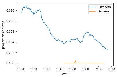
Now that we have the proportion of births, let us plot the popularity of a name through the years. How about plotting the popularity of the female names Elizabeth, and Deneen, and inspecting the underlying trends for any interesting patterns!
# Set up matplotlib for plotting in the notebook.
%matplotlib inline
import matplotlib.pyplot as plt

def plot_trends(name, sex):
    # -- YOUR CODE HERE --
    temp = bnames2[(bnames2.sex==sex) & (bnames2.name==name)]
    plt.plot(temp.year, temp.prop_births, label=name)
    plt.legend()
    plt.xlabel('year')
    plt.ylabel('proportion of births')
    return


# Plot trends for Elizabeth and Deneen
# -- YOUR CODE HERE --
plot_trends('Elizabeth', 'F')
plot_trends('Deneen', 'F')
# How many times did these female names peak?
num_peaks_elizabeth = 3
num_peaks_deneen    = 1
5. Trendy vs. Stable Names
Based on the plots we created earlier, we can see that Elizabeth is a fairly stable name, while Deneen is not. An interesting question to ask would be what are the top 5 stable and top 5 trendiest names. A stable name is one whose proportion across years does not vary drastically, while a trendy name is one whose popularity peaks for a short period and then dies down.
There are many ways to measure trendiness. A simple measure would be to look at the maximum proportion of births for a name, normalized by the sume of proportion of births across years. For example, if the name Joe had the proportions 0.1, 0.2, 0.1, 0.1, then the trendiness measure would be 0.2/(0.1 + 0.2 + 0.1 + 0.1) which equals 0.5.
Let us use this idea to figure out the top 10 trendy names in this data set, with at least a 1000 births.
# top10_trendy_names | A Data Frame of the top 10 most trendy names
names = pd.DataFrame()
name_and_sex_grouped = bnames2.groupby(['name','sex'])
names['total'] = name_and_sex_grouped['births'].sum()
#bnames2 = bnames2[bnames2.total>=1000]

names['max'] = name_and_sex_grouped['births'].max()

names = names[names.total >= 1000]

names['trendiness']=names['max']/names['total']
top10_trendy_names = names.sort_values('trendiness', ascending=False).head(10).reset_index()

top10_trendy_names
#bnames2['max'] = bnames2.groupby(['name','sex'])['births'].transform(max)
#bnames2['trendiness'] = bnames2['max']/bnames2['total']
#bnames2 = bnames2.sort_values('trendiness', ascending=False)
#bnames2.head()
#bnames_over1000 = bynames[bynames.births>=1000]
#bnames_over1000.sort_values('births')
| name | sex | total | max | trendiness | |
|---|---|---|---|---|---|
| 0 | Christop | M | 1082 | 1082 | 1.000000 |
| 1 | Royalty | F | 1057 | 581 | 0.549669 |
| 2 | Kizzy | F | 2325 | 1116 | 0.480000 |
| 3 | Aitana | F | 1203 | 564 | 0.468828 |
| 4 | Deneen | F | 3602 | 1604 | 0.445308 |
| 5 | Moesha | F | 1067 | 426 | 0.399250 |
| 6 | Marely | F | 2527 | 1004 | 0.397309 |
| 7 | Kanye | M | 1304 | 507 | 0.388804 |
| 8 | Tennille | F | 2172 | 769 | 0.354052 |
| 9 | Kadijah | F | 1411 | 486 | 0.344437 |
6. Bring in Mortality Data
So, what more is in a name? Well, with some further work, it is possible to predict the age of a person based on the name (Whoa! Really????). For this, we will need actuarial data that can tell us the chances that someone is still alive, based on when they were born. Fortunately, the SSA provides detailed actuarial life tables by birth cohorts.
| year | age | qx | lx | dx | Lx | Tx | ex | sex |
|---|---|---|---|---|---|---|---|---|
| 1910 | 39 | 0.00283 | 78275 | 222 | 78164 | 3129636 | 39.98 | F |
| 1910 | 40 | 0.00297 | 78053 | 232 | 77937 | 3051472 | 39.09 | F |
| 1910 | 41 | 0.00318 | 77821 | 248 | 77697 | 2973535 | 38.21 | F |
| 1910 | 42 | 0.00332 | 77573 | 257 | 77444 | 2895838 | 37.33 | F |
| 1910 | 43 | 0.00346 | 77316 | 268 | 77182 | 2818394 | 36.45 | F |
| 1910 | 44 | 0.00351 | 77048 | 270 | 76913 | 2741212 | 35.58 | F |
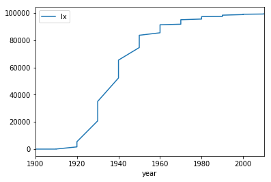
You can read the documentation for the lifetables to understand what the different columns mean. The key column of interest to us is lx, which provides the number of people born in a year who live upto a given age. The probability of being alive can be derived as lx by 100,000.
Given that 2016 is the latest year in the baby names dataset, we are interested only in a subset of this data, that will help us answer the question, "What percentage of people born in Year X are still alive in 2016?"
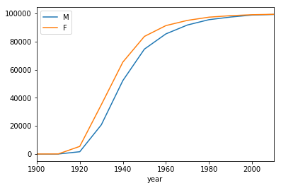
Let us use this data and plot it to get a sense of the mortality distribution!
# Read lifetables from datasets/lifetables.csv
lifetables = pd.read_csv('datasets/lifetables.csv')

# Extract subset relevant to those alive in 2016

#lifetables_2016 = lifetables[lifetables['year']+lifetables['age']==2016]

lifetables['dyear']=lifetables['year']+lifetables['age']
still_alive = lifetables[lifetables.dyear==2016]
lifetables_2016 = still_alive.drop('dyear',axis=1)
#lifetables_2016
# Plot the mortality distribution: year vs. lx
#lifetables_2016.groupby('year')['lx'].sum().plot()
lifetables_2016.plot(x='year', y='lx')
<matplotlib.axes._subplots.AxesSubplot at 0xd3ddb70>
ax = lifetables_2016[lifetables_2016.sex=='M'].plot(x='year', y='lx', label='M')
lifetables_2016[lifetables_2016.sex=='F'].plot(x='year', y='lx', label='F', ax=ax)
<matplotlib.axes._subplots.AxesSubplot at 0xd3e5780>
7. Smoothen the Curve!
We are almost there. There is just one small glitch. The cohort life tables are provided only for every decade. In order to figure out the distribution of people alive, we need the probabilities for every year. One way to fill up the gaps in the data is to use some kind of interpolation. Let us keep things simple and use linear interpolation to fill out the gaps in values of lx, between the years 1900 and 2016.
# Create smoothened lifetable_2016_s by interpolating values of lx
import numpy as np
#lifetable_2016_s = lifetables_2016.sort_values(['sex','year']).copy()
#lifetable_2016_s.interpolate(method='linear',)

year = np.arange(1900, 2016)
#year
mf = {"M": pd.DataFrame(), "F": pd.DataFrame()}
#mf
#lifetables_2016[lifetables_2016['sex'] == 'M'][["year", "lx"]].set_index('year').reindex(year).interpolate().reset_index()
for sex in ["M", "F"]:
    d = lifetables_2016[lifetables_2016['sex'] == sex][["year", "lx"]]
    mf[sex] = d.set_index('year').reindex(year).interpolate().reset_index()
    mf[sex]['sex'] = sex
#type(pd.concat(mf, ignore_index=True))
#pd.concat(mf, ignore_index=True)
lifetable_2016_s = pd.concat(mf, ignore_index = True)
lifetable_2016_s.head()
| year | lx | sex | |
|---|---|---|---|
| 0 | 1900 | 0.0 | F |
| 1 | 1901 | 6.1 | F |
| 2 | 1902 | 12.2 | F |
| 3 | 1903 | 18.3 | F |
| 4 | 1904 | 24.4 | F |
8. Distribution of People Alive by Name
Now that we have all the required data, we need a few helper functions to help us with our analysis.
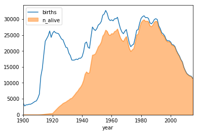
The first function we will write is get_data,which takes name and sex as inputs and returns a data frame with the distribution of number of births and number of people alive by year.
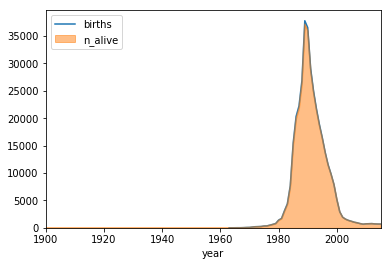
The second function is plot_name which accepts the same arguments as get_data, but returns a line plot of the distribution of number of births, overlaid by an area plot of the number alive by year.
Using these functions, we will plot the distribution of births for boys named Joseph and girls named Brittany.
def get_data(name, sex):
       # YOUR CODE HERE
    bnames_name_sex = bnames[(bnames.name==name)&(bnames.sex==sex)]
    lifetable_2016_s_sex = lifetable_2016_s[lifetable_2016_s.sex == sex]
    data = pd.merge(lifetable_2016_s_sex, bnames_name_sex, how='left', on='year')
    data['n_alive'] = data['lx']*data['births']/100000
    data = data.drop(['sex_y'], axis=1)
    data = data[['name', 'sex_x', 'births', 'year', 'lx', 'n_alive']]
    #print(data)
    return data


def plot_data(name, sex):
    # YOUR CODE HERE
    ax = get_data(name,sex).plot(x='year', y='births')
    get_data(name,sex).plot(kind='area',alpha=0.5, x='year', y='n_alive', ax=ax)
    return

# Plot the distribution of births and number alive for Joseph and Brittany
plot_data('Joseph','M')
plot_data('Brittany','F')
#bnames
#lifetable_2016_s
9. Estimate Age
In this section, we want to figure out the probability that a person with a certain name is alive, as well as the quantiles of their age distribution. In particular, we will estimate the age of a female named Gertrude. Any guesses on how old a person with this name is? How about a male named William?
# Import modules
from wquantiles import quantile

# Function to estimate age quantiles
def estimate_age(name, sex):
    # YOUR CODE HERE
    data = get_data(name,sex)
    data = data.fillna(0)
    qs = [0.25, 0.5, 0.75]
    quantiles = [2016 - int(quantile(data.year, data.n_alive, q)) for q in qs]
    p_alive = data.n_alive.sum()/data.births.sum()
    #data['age']=2016-data['year']
    result = pd.Series(index=['name','p_alive','q25','q50','q75','sex'])
    result['name']=name
    result['p_alive']=p_alive
    result['q25']=quantiles[0]
    result['q50']=quantiles[1]
    result['q75']=quantiles[2]
    result['sex']=sex

    return result

# Estimate the age of Gertrude
estimate_age('Gertrude', 'F')

#  result = dict(zip(['q25', 'q50', 'q75'], quantiles))
#  result['p_alive'] = round(data.n_alive.sum()/data.births.sum()*100, 2)
#  result['sex'] = sex
#  result['name'] = name
#  return pd.Series(result)
10. Median Age of Top 10 Female Names
In the previous section, we estimated the age of a female named Gertrude. Let's go one step further this time, and compute the 25th, 50th and 75th percentiles of age, and the probability of being alive for the top 10 most common female names of all time. This should give us some interesting insights on how these names stack up in terms of median ages!
# Create median_ages: DataFrame with Top 10 Female names,
#    age percentiles and probability of being alive
# -- YOUR CODE HERE --

#sex='F'
#bnames_agg = bnames.groupby(['sex', 'name'], as_index=False)['births'].sum()
#top_ten_female = bnames_agg.sort_values(['sex','births'], ascending=[True, False]).head(10).name
#top_ten_female

#for name in top_ten_female:
    #estimate_age(name, sex)
#    print(name, sex)


top_10_female_names = bnames.\
    groupby(['sex', 'name'], as_index = False).\
    agg({'births': np.sum}).\
    sort_values('births', ascending = False).\
    query('sex == "F"').\
    head(10).\
    reset_index(drop = True)
estimates = pd.concat([estimate_age(name, 'F') for name in top_10_female_names.name], axis = 1)
median_ages = estimates.T.sort_values('q50').reset_index(drop = True)
median_ages
#estimate_age('Jennifer','F')